NVBUG Literature Clustering
Data Pre-processing
create a function that will process the text data for us
For this purpose we will be using the spacy library. This function will convert text to lower case, remove punctuation, and find and remove stopwords. For the parser, we will use en_core_sci_lg. This is a model for processing biomedical, scientific or clinical text.
sentence = "Hi Sheng/Thejesvi,In our 7nm C&C, we found there are many H360.FB.W.1.1 violations location at corner edge cells:"
mytokens = parser(sentence)
print (mytokens)
mytokens = [ word.lemma_.lower().strip() if word.lemma_ != "-PRON-" else word.lower_ for word in mytokens ]
print (mytokens)
mytokens = [ word for word in mytokens if word not in stopwords and word not in punctuations ]
print (mytokens)
mytokens = " ".join([i for i in mytokens])
print (mytokens)


Hi Sheng/Thejesvi,In our 7nm C&C, we found there are many H360.FB.W.1.1 violations location at corner edge cells:
['hi', 'sheng/thejesvi', ',', 'in', 'our', '7', 'nm', 'c&c', ',', 'we', 'find', 'there', 'be', 'many', 'h360.fb.w.1.1', 'violation', 'location', 'at', 'corner', 'edge', 'cell', ':']
['hi', 'sheng/thejesvi', '7', 'nm', 'c&c', 'find', 'h360.fb.w.1.1', 'violation', 'location', 'corner', 'edge', 'cell']
hi sheng/thejesvi 7 nm c&c find h360.fb.w.1.1 violation location corner edge cell
text2 = meta_df['processed_text'].values[4:7]
text2
array(['net route layer tm1 1.2075 m5a 3.4200 m4a 2.0940 m3a 3.5600 m2 1.5400',
'devjani chatterjee subject ga100:revp1.0:vialadder addition hier macro hi preeti try insert ladder ckbd cell hier macro able insert ladder cell input pin ckbd48 cell ladder insert find log file /home/scratch.devjanic_gpu_1/ga100/nvgpu_ga100/layout/revp1.0/pandr/hier_macros/socialprime/nv_gaa_fbp_clk_entry/via_ladder_analysis/logs/nv_gaa_fbp_clk_entry.ipo1007.run.plan.place.04_10_07_51.log db:/home/scratch.devjanic_gpu_1/ga100/nvgpu_ga100/layout/revp1.0/pandr/hier_macros/socialprime/nv_gaa_fbp_clk_entry/via_ladder_analysis/nv_gaa_fbp_clk_entry.nlib/nv_gaa_fbp_clk_entry_ipo1007_place proc nvb_create_area_pins_for_anc care hier macro good snapshot',
'hi yi filing bug track region cts icc2 7 nm let know testcase test gv100 netlists map 7 nm jayanth provide need thanks umang'],
dtype=object)
meta_df['processed_text'].apply(lambda x: len(x.strip().split()))[4:7]
5 13
6 38
7 24
Name: processed_text, dtype: int64
1
vectorizer = TfidfVectorizer()
X = vectorizer.fit_transform(text2)
print(vectorizer.get_feature_names())
print(len(vectorizer.get_feature_names()))
['04_10_07_51', '0940', '2075', '4200', '5400', '5600', 'able', 'addition', 'bug', 'care', 'cell', 'chatterjee', 'ckbd', 'ckbd48', 'cts', 'db', 'devjani', 'devjanic_gpu_1', 'file', 'filing', 'find', 'ga100', 'good', 'gv100', 'hi', 'hier', 'hier_macros', 'home', 'icc2', 'input', 'insert', 'ipo1007', 'jayanth', 'know', 'ladder', 'layer', 'layout', 'let', 'log', 'logs', 'm2', 'm3a', 'm4a', 'm5a', 'macro', 'map', 'need', 'net', 'netlists', 'nlib', 'nm', 'nv_gaa_fbp_clk_entry', 'nv_gaa_fbp_clk_entry_ipo1007_place', 'nvb_create_area_pins_for_anc', 'nvgpu_ga100', 'pandr', 'pin', 'place', 'plan', 'preeti', 'proc', 'provide', 'region', 'revp1', 'route', 'run', 'scratch', 'snapshot', 'socialprime', 'subject', 'test', 'testcase', 'thanks', 'tm1', 'track', 'try', 'umang', 'via_ladder_analysis', 'vialadder', 'yi']
X
<3x80 sparse matrix of type '<class 'numpy.float64'>'
with 81 stored elements in Compressed Sparse Row format>
X.toarray()
array([[0. , 0.2773501 , 0.2773501 , 0.2773501 , 0.2773501 ,
0.2773501 , 0. , 0. , 0. , 0. ,
0. , 0. , 0. , 0. , 0. ,
0. , 0. , 0. , 0. , 0. ,
0. , 0. , 0. , 0. , 0. ,
0. , 0. , 0. , 0. , 0. ,
0. , 0. , 0. , 0. , 0. ,
0.2773501 , 0. , 0. , 0. , 0. ,
0.2773501 , 0.2773501 , 0.2773501 , 0.2773501 , 0. ,
0. , 0. , 0.2773501 , 0. , 0. ,
0. , 0. , 0. , 0. , 0. ,
0. , 0. , 0. , 0. , 0. ,
0. , 0. , 0. , 0. , 0.2773501 ,
0. , 0. , 0. , 0. , 0. ,
0. , 0. , 0. , 0.2773501 , 0. ,
0. , 0. , 0. , 0. , 0. ],
[0.08231682, 0. , 0. , 0. , 0. ,
0. , 0.08231682, 0.08231682, 0. , 0.08231682,
0.24695047, 0.08231682, 0.08231682, 0.08231682, 0. ,
0.08231682, 0.08231682, 0.16463365, 0.08231682, 0. ,
0.08231682, 0.24695047, 0.08231682, 0. , 0.06260407,
0.24695047, 0.16463365, 0.16463365, 0. , 0.08231682,
0.24695047, 0.08231682, 0. , 0. , 0.24695047,
0. , 0.16463365, 0. , 0.16463365, 0.08231682,
0. , 0. , 0. , 0. , 0.24695047,
0. , 0. , 0. , 0. , 0.08231682,
0. , 0.32926729, 0.08231682, 0.08231682, 0.16463365,
0.16463365, 0.08231682, 0.08231682, 0.08231682, 0.08231682,
0.08231682, 0. , 0. , 0.24695047, 0. ,
0.08231682, 0.16463365, 0.08231682, 0.16463365, 0.08231682,
0. , 0. , 0. , 0. , 0. ,
0.08231682, 0. , 0.16463365, 0.08231682, 0. ],
[0. , 0. , 0. , 0. , 0. ,
0. , 0. , 0. , 0.20594101, 0. ,
0. , 0. , 0. , 0. , 0.20594101,
0. , 0. , 0. , 0. , 0.20594101,
0. , 0. , 0. , 0.20594101, 0.15662345,
0. , 0. , 0. , 0.20594101, 0. ,
0. , 0. , 0.20594101, 0.20594101, 0. ,
0. , 0. , 0.20594101, 0. , 0. ,
0. , 0. , 0. , 0. , 0. ,
0.20594101, 0.20594101, 0. , 0.20594101, 0. ,
0.41188202, 0. , 0. , 0. , 0. ,
0. , 0. , 0. , 0. , 0. ,
0. , 0.20594101, 0.20594101, 0. , 0. ,
0. , 0. , 0. , 0. , 0. ,
0.20594101, 0.20594101, 0.20594101, 0. , 0.20594101,
0. , 0.20594101, 0. , 0. , 0.20594101]])
Vectorization
https://scikit-learn.org/stable/modules/generated/sklearn.feature_extraction.text.TfidfVectorizer.html
Now that we have pre-processed the data, it is time to convert it into a format that can be handled by our algorithms. For this purpose we will be using tf-idf. This will convert our string formatted data into a measure of how important each word is to the instance out of the literature as a whole.
>>> from sklearn.feature_extraction.text import CountVectorizer
>>> corpus = [
...     'This is the first document.',
...     'This document is the second document.',
...     'And this is the third one.',
...     'Is this the first document?',
... ]
>>> vectorizer = CountVectorizer()
>>> X = vectorizer.fit_transform(corpus)
>>> print(vectorizer.get_feature_names())
['and', 'document', 'first', 'is', 'one', 'second', 'the', 'third', 'this']
>>> print(X.toarray())
[[0 1 1 1 0 0 1 0 1]
 [0 2 0 1 0 1 1 0 1]
 [1 0 0 1 1 0 1 1 1]
 [0 1 1 1 0 0 1 0 1]]
PCA & Clustering
https://scikit-learn.org/stable/modules/generated/sklearn.decomposition.PCA.html
Let's see how much we can reduce the dimensions while still keeping 95% variance. We will apply Principle Component Analysis (PCA) to our vectorized data. The reason for this is that by keeping a large number of dimensions with PCA, you don’t destroy much of the information, but hopefully will remove some noise/outliers from the data, and make the clustering problem easier for k-means. Note that X_reduced will only be used for k-means, t-SNE will still use the original feature vector X that was generated through tf-idf on the NLP processed text.
from sklearn.decomposition import PCA

pca = PCA(n_components=0.95, random_state=42)
X_reduced= pca.fit_transform(X.toarray())
X_reduced.shape
(3, 2)
X_reduced
array([[ 8.17829820e-01, -8.02721901e-16],
       [-4.08914910e-01, -7.03631557e-01],
       [-4.08914910e-01,  7.03631557e-01]])
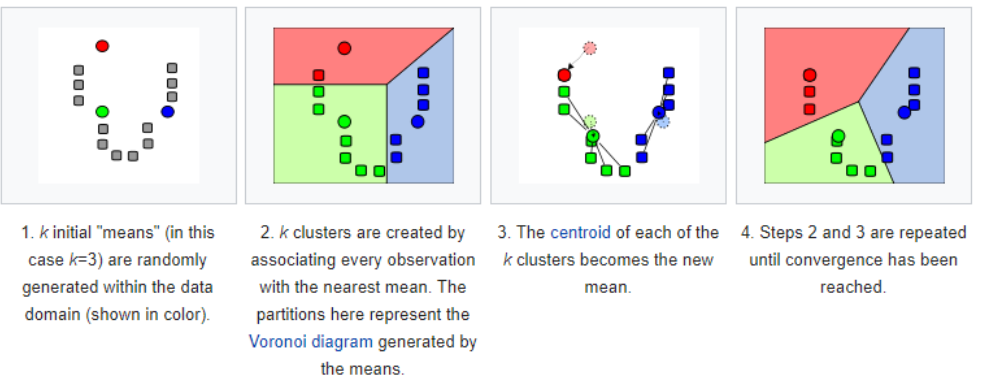
To separate the literature, k-means will be run on the vectorized text. Given the number of clusters, k, k-means will categorize each vector by taking the mean distance to a randomly initialized centroid. The centroids are updated iteratively.
https://en.wikipedia.org/wiki/K-means_clustering
from sklearn.cluster import KMeans
How many clusters?
To find the best k value for k-means we'll look at the distortion at different k values. Distortion computes the sum of squared distances from each point to its assigned center. When distortion is plotted against k there will be a k value after which decreases in distortion are minimal. This is the desired number of clusters.
k_means = KMeans(n_clusters=2, random_state=42).fit(X_reduced)
print(k_means)
KMeans(algorithm='auto', copy_x=True, init='k-means++', max_iter=300,
       n_clusters=2, n_init=10, n_jobs=None, precompute_distances='auto',
       random_state=42, tol=0.0001, verbose=0)
 k_means.fit(X_reduced)
KMeans(algorithm='auto', copy_x=True, init='k-means++', max_iter=300,
       n_clusters=2, n_init=10, n_jobs=None, precompute_distances='auto',
       random_state=42, tol=0.0001, verbose=0)
print (X_reduced)
[[ 8.17829820e-01 -8.02721901e-16]
 [-4.08914910e-01 -7.03631557e-01]
 [-4.08914910e-01  7.03631557e-01]]

print (k_means.cluster_centers_)
[[-4.08914910e-01  2.96059473e-16]
 [ 8.17829820e-01 -8.02721901e-16]]

cdist(X_reduced, k_means.cluster_centers_, 'euclidean')
array([[1.22674473, 0.        ],
       [0.70363156, 1.41421356],
       [0.70363156, 1.41421356]])

np.min(cdist(X_reduced, k_means.cluster_centers_, 'euclidean'), axis=1)
array([0.        , 0.70363156, 0.70363156])

sum(np.min(cdist(X_reduced, k_means.cluster_centers_, 'euclidean'), axis=1))/X.shape[0]
0.4690877045277359


k_means = KMeans(n_clusters=3, random_state=42).fit(X_reduced)
print(k_means)
KMeans(algorithm='auto', copy_x=True, init='k-means++', max_iter=300,
       n_clusters=3, n_init=10, n_jobs=None, precompute_distances='auto',
       random_state=42, tol=0.0001, verbose=0)
k_means.fit(X_reduced)
KMeans(algorithm='auto', copy_x=True, init='k-means++', max_iter=300,
       n_clusters=3, n_init=10, n_jobs=None, precompute_distances='auto',
       random_state=42, tol=0.0001, verbose=0)

print (X_reduced)
[[ 8.17829820e-01 -8.02721901e-16]
 [-4.08914910e-01 -7.03631557e-01]
 [-4.08914910e-01  7.03631557e-01]]
print (k_means.cluster_centers_)
[[-4.08914910e-01 -7.03631557e-01]
 [ 8.17829820e-01 -8.02721901e-16]
 [-4.08914910e-01  7.03631557e-01]]

cdist(X_reduced, k_means.cluster_centers_, 'euclidean')
array([[1.41421356, 0.        , 1.41421356],
       [0.        , 1.41421356, 1.40726311],
       [1.40726311, 1.41421356, 0.        ]])

np.min(cdist(X_reduced, k_means.cluster_centers_, 'euclidean'), axis=1)
array([0., 0., 0.])
Run k-means
Now that we have an appropriate k value, we can run k-means on the PCA-processed feature vector (X_reduced).
# run kmeans with many different k
distortions = []
K = range(2, 4)
for k in K:
    k_means = KMeans(n_clusters=k, random_state=42).fit(X_reduced)
    k_means.fit(X_reduced)
    distortions.append(sum(np.min(cdist(X_reduced, k_means.cluster_centers_, 'euclidean'), axis=1)) / X.shape[0])
    #print('Found distortion for {} clusters'.format(k))

X_line = [K[0], K[-1]]
Y_line = [distortions[0], distortions[-1]]

# Plot the elbow
plt.plot(K, distortions, 'b-')
plt.plot(X_line, Y_line, 'r')
plt.xlabel('k')
plt.ylabel('Distortion')
plt.title('The Elbow Method showing the optimal k')
plt.show()
Dimensionality Reduction with t-SNE
t-Distributed Stochastic Neighbor Embedding (t-SNE) is a (prize-winning) technique for dimensionality reduction that is particularly well suited for the visualization of high-dimensional datasets. The technique can be implemented via Barnes-Hut approximations, allowing it to be applied on large real-world datasets. We applied it on data sets with up to 30 million examples. The technique and its variants are introduced in the following papers:
Using t-SNE https://lvdmaaten.github.io/tsne/ we can reduce our high dimensional features vector to 2 dimensions. By using the 2 dimensions as x,y coordinates, the body_text can be plotted.
t-Distributed Stochastic Neighbor Embedding (t-SNE) reduces dimensionality while trying to keep similar instances close and dissimilar instances apart. It is mostly used for visualization, in particular to visualize clusters of instances in high-dimensional space
Cite: Hands-On Machine Learning with Scikit-Learn, Keras & TensorFlow: Second Edition | Aurélien Geron https://github.com/ageron/handson-ml2
from sklearn.manifold import TSNE

tsne = TSNE(verbose=1, perplexity=100, random_state=42)
X_embedded = tsne.fit_transform(X.toarray())

[t-SNE] Computing 2 nearest neighbors...
[t-SNE] Indexed 3 samples in 0.001s...
[t-SNE] Computed neighbors for 3 samples in 0.000s...
[t-SNE] Computed conditional probabilities for sample 3 / 3
[t-SNE] Mean sigma: 1125899906842624.000000
[t-SNE] KL divergence after 250 iterations with early exaggeration: 31.644199
[t-SNE] KL divergence after 450 iterations: 0.000000

X_embedded
array([[ -18.833384, -276.80054 ],
       [-210.60179 ,  143.00536 ],
       [-478.27985 , -232.9741  ]], dtype=float32)
So that step took a while! Let's take a look at what our data looks like when compressed to 2 dimensions.
from matplotlib import pyplot as plt
import seaborn as sns

# sns settings
sns.set(rc={'figure.figsize':(5,5)})

# colors
palette = sns.color_palette("bright", 1)

# plot
sns.scatterplot(X_embedded[:,0], X_embedded[:,1], palette=palette)
plt.title('t-SNE with no Labels')
plt.savefig("t-sne_df_test.png")
plt.show()
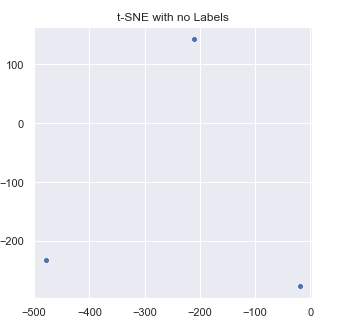
This looks pretty bland. There are some clusters we can immediately detect, but the many instances closer to the center are harder to separate. t-SNE did a good job at reducing the dimensionality, but now we need some labels. Let's use the clusters found by k-means as labels. This will help visually separate different concentrations of topics.
%matplotlib inline
from matplotlib import pyplot as plt
import seaborn as sns

# sns settings
sns.set(rc={'figure.figsize':(5,5)})

# colors
palette = sns.hls_palette(3, l=.4, s=.9)

# plot
sns.scatterplot(X_embedded[:,0], X_embedded[:,1], hue=y_pred, legend='full', palette=palette)
plt.title('t-SNE with Kmeans Labels')
plt.savefig("improved_cluster_tsne.png")
plt.show()
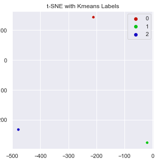
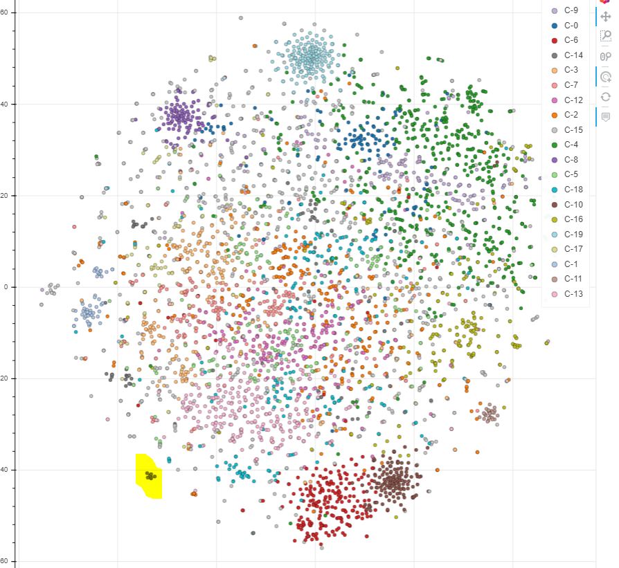
The labeled plot gives better insight into how the papers are grouped. It is interesting that both k-means and t-SNE are able to agree on certain clusters even though they were ran independetly. The location of each paper on the plot was determined by t-SNE while the label (color) was determined by k-means. If we look at a particular part of the plot where t-SNE has grouped many articles forming a cluster, it is likely that k-means is uniform in the labeling of this cluster (most of the cluster is the same color). This behavior shows that structure within the literature can be observed and measured to some extent.
Now there are other cases where the colored labels (k-means) are spread out on the plot (t-SNE). This is a result of t-SNE and k-means finding different connections in the higher dimensional data. The topics of these papers often intersect so it hard to cleanly separate them. This effect can be observed in the formation of subclusters on the plot. These subclusters are a conglomeration of different k-means labels but may share some connection determined by t-SNE.
This organization of the data does not act as a simple search engine. The clustering + dimensionality reduction is performed on the mathematical similarities of the publications. As an unsupervised approach, the algorithms may even find connections that were unnaparent to humans. This may highlight hidden shared information and advance further research.
Topic Modeling on Each Cluster
Now we will attempt to find the most significant words in each clusters. K-means clustered the articles but did not label the topics. Through topic modeling we will find out what the most important terms for each cluster are. This will add more meaning to the cluster by giving keywords to quickly identify the themes of the cluster.
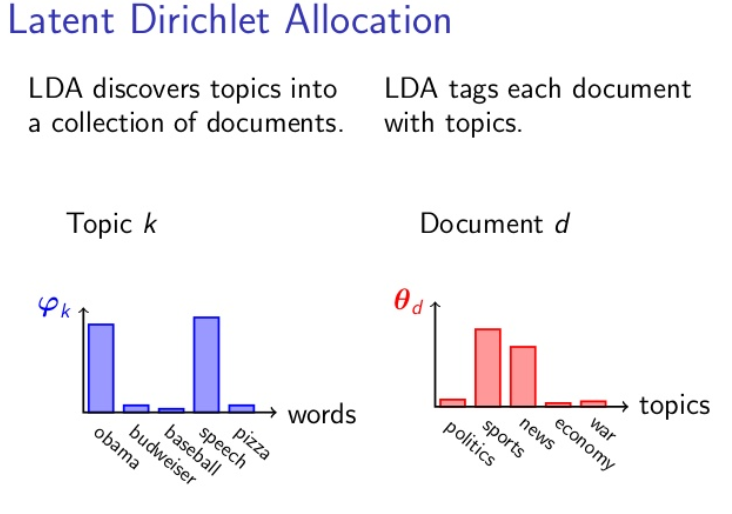
For topic modeling, we will use LDA (Latent Dirichlet Allocation). In LDA, each document can be described by a distribution of topics and each topic can be described by a distribution of words.
from sklearn.decomposition import LatentDirichletAllocation
from sklearn.feature_extraction.text import CountVectorizer
>>> from sklearn.feature_extraction.text import CountVectorizer
>>> corpus = [
...     'This is the first document.',
...     'This document is the second document.',
...     'And this is the third one.',
...     'Is this the first document?',
... ]
>>> vectorizer = CountVectorizer()
>>> X = vectorizer.fit_transform(corpus)
>>> print(vectorizer.get_feature_names())
['and', 'document', 'first', 'is', 'one', 'second', 'the', 'third', 'this']
>>> print(X.toarray())
[[0 1 1 1 0 0 1 0 1]
 [0 2 0 1 0 1 1 0 1]
 [1 0 0 1 1 0 1 1 1]
 [0 1 1 1 0 0 1 0 1]]
>>> vectorizer2 = CountVectorizer(analyzer='word', ngram_range=(2, 2))
>>> X2 = vectorizer2.fit_transform(corpus)
>>> print(vectorizer2.get_feature_names())
['and this', 'document is', 'first document', 'is the', 'is this',
'second document', 'the first', 'the second', 'the third', 'third one',
 'this document', 'this is', 'this the']
 >>> print(X2.toarray())
 [[0 0 1 1 0 0 1 0 0 0 0 1 0]
 [0 1 0 1 0 1 0 1 0 0 1 0 0]
 [1 0 0 1 0 0 0 0 1 1 0 1 0]
 [0 0 1 0 1 0 1 0 0 0 0 0 1]]
vectorizer_test = CountVectorizer(min_df=5, max_df=0.9, stop_words='english', lowercase=True, token_pattern='[a-zA-Z\-][a-zA-Z\-]{2,}')

vectorizer_test.fit_transform(meta_df.loc[meta_df['y'] == 0, 'processed_text'])
print(len(vectorizer_test.get_feature_names()))
756

vectorizer_test2 = CountVectorizer(min_df=5, max_df=0.9, stop_words='english', lowercase=True)

vectorizer_test2.fit_transform(meta_df.loc[meta_df['y'] == 0, 'processed_text'])
print(len(vectorizer_test2.get_feature_names()))
682
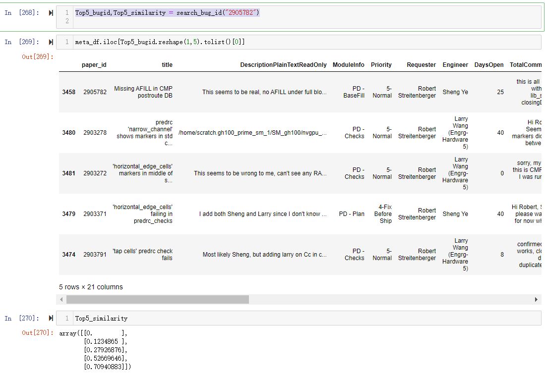
https://nvbugswb.nvidia.com/NVBugs5/MethodologyBug.aspx?isCad=true&bugid=2905782 https://nvbugswb.nvidia.com/NVBugs5/MethodologyBug.aspx?isCad=true&bugid=2903278
Hi Robert,
Seems the markers did flag between RAMs, and I suspect that it should be similar to the bug 2903272, please help double confirm.
https://nvbugswb.nvidia.com/NVBugs5/MethodologyBug.aspx?isCad=true&bugid=2903272
df cheatsheet
pattern = meta_df.loc[meta_df['y'] == 0, 'processed_text'].str.contains('sys')
print('pattern : \n', pattern)
filter_data = meta_df.loc[meta_df['y'] == 0, 'processed_text'][pattern]
print('filter data : \n', filter_data)
pattern :
 1       False
9       False
11      False
31      False
44      False
        ...
4947    False
4954    False
4991    False
4997     True
5015    False
Name: processed_text, Length: 230, dtype: bool
filter data :
 130     similar previous time early_cts fix previous c...
141     place region root cgs ccm center time path cg ...
273     simon feasible change follow command gen tcl s...
369     yi observe design icc unable utilize slack pos...
426     tracking use amogh highlight late seahawk fast...
                              ...
4747    pp flow setup path ram_access_max__ssg_c_pv_bi...
4760    karthik find eco change dump final icc eco cha...
4927    continue max_transition violation place icc_sh...
4932    buffer insert datum path postroute cause setup...
4997    yi check cts stage opt ssg_c_pv_bin_opt_max_si...
Name: processed_text, Length: 62, dtype: object
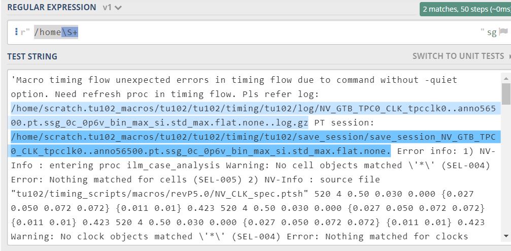
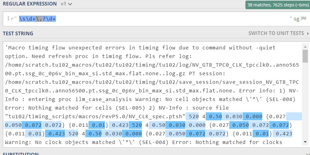
regexp https://regex101.com/r/yS7lG7/1